Top 5 Statistical Techniques in Python

[scastle]

A data scientist must be skilled in many arts: math and statistics, computer science, and domain knowledge. No matter your skill, career level, or title, the ability to analyze, organize, and visualize data are vital skills in our world of quickly growing and ever-changing data. 

Statistics and programming go hand in hand. Mastering statistical techniques and knowing how to implement them via a programming language are essential building blocks for advanced analytics. In this article, we will explain how to execute five statistical techniques using Python.

Importance of statistical techniques

Before proceeding to the how-to sections, let’s briefly cover what statistical techniques are used for and why they’re so important:

• Finding relationships between variables in data: Statistical techniques can help us find correlations between various features of data and target relationships between those features, leading to a better understanding of the problem to be solved.
• Summarizing and analyzing data: With a better understanding of a dataset, it’s easy to analyze and summarize it, as well as extract insights from complex information.
• Interpreting better results: Statistical techniques allow users to make predictions for unseen data, more easily improving the accuracy of output and results.
• Applying appropriate machine learning (ML) models: Different ML techniques are better suited for different types of problems. This can often only be judged with good knowledge of various statistical methods.
• Transforming observations into information: Observing data and finding solutions is different from conveying them accurately. It’s easy to transform various observations to simplified and significant insights using statistical methods.

Statistical techniques to handle non trivial data

There are many statistical techniques to choose from when handling non trivial data. Let’s discuss five specific statistical techniques that are very efficient in handling this kind of data.

1. Linear regression

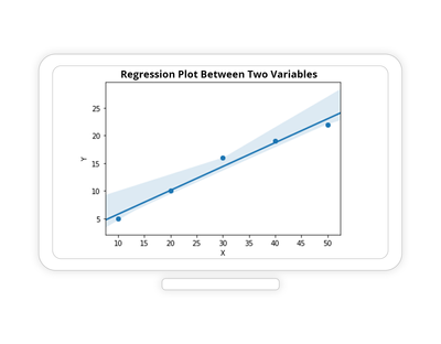
Linear regression is an estimated relationship between two or more variables. It shows the linear relationship between the dependent variable (Y) and the independent variable (X). In this technique, the dependent variable and the independent variable(s) are continuous, and the nature of the regression line is linear. A regression line is the best fit straight line.

Linear regression is a form of supervised learning (or predictive modeling). In supervised learning, the dependent variable is predicted from the combination of independent variables. 

When a single independent variable is used to predict the value of a dependent variable, it’s called simple linear regression. In cases where two or more independent variables are used to predict the value of a dependent variable, it’s called multiple linear regression.

Linear regression is represented by equation Y=b*X + a + e, where a is the intercept, b is the slope of the line, and e is the error term.

Practical applications of linear regression:

• Predicting sales of a product based on pricing, performance, risk, market performance, and other parameters
• Real-time server load prediction for cloud computing services
• Market research studies and customer survey analysis
• Determining the ROI of a new policy, initiative, or campaign

Code:

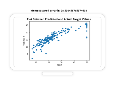
Let’s see a Python code implementation of linear regression on a Boston house-prices dataset to determine the price of houses at various places in Boston with respect to 13 features like per capita crime rate by town, proportion of non-retail business acres per town, the age of people who own the house, etc. In the code, test_x is a data frame of 13 features, and test_y is the target variable (price of houses):

from sklearn.linear_model import LinearRegression
lin_reg = LinearRegression(normalize=True)
pred = lin_reg.predict(test_x)
MSE=mean_squared_error(test_y, pred)
print("Mean Squared Error is: ", MSE)
plt.scatter(test_y, pred)
plt.xlabel('Test Y')
plt.ylabel('Predicted Y')
plt.title("Plot between Predicted and Actual target values")
plt.show()

From the above graph, we can see that there’s not much difference between the actual and predicted prices of houses in Boston. Also, the mean squared error is also not much; mean squared error is the regression loss, which we have calculated between predicted and actual values. Regression loss is the loss that occurs when we try to draw a best fit straight regression line in the above graph. 

We can draw a sample table to compare actual and predicted values for better understanding. We can see that predicted values are close to actual values. Hence, we can say our regression model of Boston housing prices seems to work pretty well.

Actual	Predicted
23.1	24.369364
32.2	31.614934
10.8	11.422104
23.1	24.928622
21.2	23.311708
22.2	22.776408
24.1	20.650812
17.3	16.035198
7.0	7.079786

2. Logistic regression

Logistic regression is a classification technique that categorizes the dependent variable into multiple categorical classes (i.e., discrete values based on independent variables). It is also a supervised learning technique borrowed from the field of statistics. It is used for classification only when the dependent variable is categorical. 

When the target label is numerical, use linear regression, and when the target label is binary or discrete, use logistic regression.

Classification is divided into two types on the basis of the number of output classes: Binary classification has two output classes, and multi-class classification has multiple output classes.

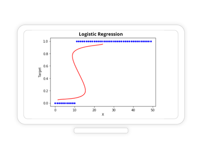
Logistic regression aims to find the plane that separates the classes in the best possible way. Logistic regression divides its output using the logistic Sigmoid function, which returns a probability value. See the diagram below of logistic regression with Sigmoid function.

Practical applications of classification:

• Predictive lead scoring to increase sales revenue
• Customer churn likelihood prediction

Code:

Let’s see Python code implementation of logistic regression on an Amazon fine food reviews dataset. This dataset consists of reviews of fine foods from Amazon over a period of more than 10 years. We are analyzing text of reviews to determine whether a given review is positive or negative:

BOW_train and BOW_test are input data after CountVectoriation of review text. Y_train and y_test is the target variable of the training and test datasets.

#Apply Logistic Regression Modeling
log_model = LogisticRegression()
log_model.fit(BOW_train, y_train)


#Calculate accuracy score
print("Accuracy score of Logistic Regression: ",log_model.score(BOW_test,y_test))


#Calculate Confusion Matrix
pred=log_model.predict(BOW_test)
df_cm = pd.DataFrame(confusion_matrix(y_test,pred),  range(2),range(2))    
sns.heatmap(df_cm, annot=True, cmap='YlGn', annot_kws={"size": 20},fmt='g')# font size
plt.title("Confusion Matrix")
plt.xlabel("Predicted Label")
plt.ylabel("True Label")
plt.show()

The accuracy score is calculated to check the accuracy of logistic regression. We have predicted review text with 91.27% accuracy via logistic regression.

A confusion matrix has also been drawn for logistic regression. The confusion matrix is a performance analysis metric that defines the code’s ability to accurately predict positive and negative reviews.

Here, we can see 97,779 were true positive values, meaning that 97,779 positive reviews were correctly predicted as positive, and 2,219 positive reviews were predicted as negative reviews (these are called false positives). Positive reviews were predicted with 97.78% accuracy.

Of the negative reviews, 11,910 were true negatives, meaning that 11,910 negative reviews were correctly predicted as negative, and 8,269 negative reviews were predictive as positive (these are called false negatives). Negative reviews were predicted with 59.02% accuracy.

3. Tree-based techniques

Tree-based techniques are for decision-making. They aid in these processes by viewing decisions at a particular point based on the given information that will yield the greatest positive outcome. This approach is widely used and practical as it models the way we humans approach a problem.

These tree-based statistical techniques can be used for both regression and classification problems. Based on independent variables, the tree is split to create branches. This method works very well with nonlinear relationships, unlike linear regression.

Practical applications of tree-based techniques:

• Customer relationship management
• Credit scoring modeling

Decision tree

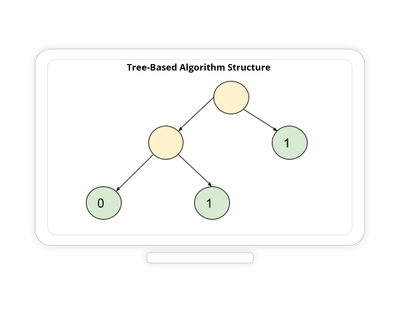
A decision tree is a supervised ML algorithm used for both categorical and continuous input and output variables. The decision tree starts with one node and then divides into several. It can also be understood as a nested “if-else” structure. 

Code:

Let’s see Python code implementation of a decision tree on the Amazon fine food reviews dataset to determine whether the review text of fine food on Amazon is positive or negative:

from sklearn.tree import DecisionTreeClassifier
model_DT = DecisionTreeClassifier()
model_DT.fit(BOW_train, y_train)
print("Accuracy score of Decision Tree: ",model_DT.score(BOW_test,y_test))
pred=model_DT.predict(BOW_test)
df_cm = pd.DataFrame(confusion_matrix(y_test,pred),  range(2),range(2))    
sns.heatmap(df_cm, annot=True, cmap='YlGn', annot_kws={"size": 20},fmt='g')# font size
plt.title("Confusion Matrix")
plt.xlabel("Predicted Label")
plt.ylabel("True Label")
plt.show()

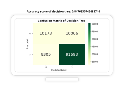
An accuracy score is calculated to check the accuracy of the decision tree. We can see that 84% of review text is predicted correctly, meaning 84% of positive reviews were correctly predicted as positive, and negative reviews predicted negative.

A confusion matrix is also drawn for our decision tree. Here, we can see 91,693 are true positive values, meaning that 91,693 positive reviews were correctly predicted as positive, and 8,305 positive reviews were predicted as negative reviews (false positives).

On the negative side, 10,173 were true negatives (meaning 10,173 negative reviews were predicted correctly as negative), and 10,006 negative reviews were predicted positive (false negatives).

We can see clearly the decision tree works very well in predicting positive reviews correctly, with about 92% accurate predictions ((91693/(91693+8305))*100).

Bagging

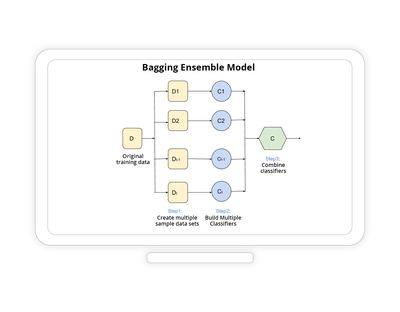
Bagging is an ensemble model that uses a combination of different models on different sample datasets of training data. In bagging, multiple homogeneous models (often called “weak learners”) are trained parallelly to solve the same problem and combined to get better results.

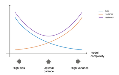
Every model tries to achieve low bias and low variance, although they often vary in opposite directions. The aim is to create a robust model that avoids both high variance and high bias. This is known as the bias-variance tradeoff as shown in the diagram below: 

Bagging is one way to decrease the variance of your predicting model by generating sample data from training data. Every sample dataset is modeled independently using weak learners, and then the results of these multiple classifiers modeled on different sub-samples of the same dataset are combined. Bagging is more robust than the single model implementation. 

One disadvantage of bagging is that it introduces a loss of interpretability of a model. Bagging may lead to lots of bias when the proper procedure is ignored. Despite bagging being highly accurate, it can be computationally expensive. 

Whenever our aim is to reduce variance (not bias), we can use bagging; it’s suitable for high-variance, low-bias models. Never use bagging when you have low-variance and high-bias models.

Practical applications of bagging: 

• E-commerce: Will a customer buy the product or not?
• Finance: Detect whether a customer will pay debt on time or not

A random forest is an example of bagging implementation.

Code:

Let’s see Python code implementation of a random forest on the Amazon fine food reviews dataset to determine whether the review text of fine food on Amazon is positive or negative:

from sklearn.ensemble import RandomForestClassifier
model_RF = RandomForestClassifier()
model_RF.fit(BOW_train, y_train)
print("Accuracy score of Random Forest: ",model_DT.score(BOW_test,y_test))
pred=model_RF.predict(BOW_test)
df_cm = pd.DataFrame(confusion_matrix(y_test,pred), range(2),range(2))    
sns.heatmap(df_cm, annot=True, cmap='YlGn', annot_kws={"size": 20},fmt='g')# font size
plt.title("Confusion Matrix")
plt.xlabel("Predicted Label")
plt.ylabel("True Label")
plt.show()

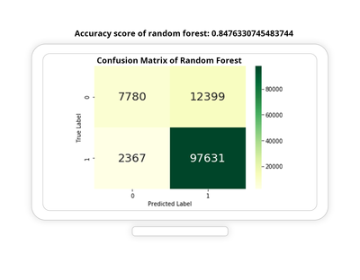
The accuracy score is calculated to check the accuracy of the random forest. Our accuracy score of 0.8476 tells us that 84.76% of reviews are predicted correctly.

A confusion matrix is also drawn for a random forest. With this confusion matrix, we can see that the predicted accuracy of positive and negative reviews varies. The confusion matrix tells us that 97.63% of positive reviews were predicted correctly, and 38.55% of negative reviews were predicted correctly. We can see in the confusion matrix that true positive prediction improved with the random forest technique compared to decision trees.

Boosting

Boosting calculates outputs using a family of algorithms and then averaging the result using a weighted average approach. Boosting uses multiple weak learners sequentially in a very adaptative way such that each model in the sequence gives more importance to observations in the dataset that were badly handled by the previous models in the sequence. At the end of the boosting process, a strong learner is obtained with reduced bias.

Boosting works very well inside the context of the bias-variance tradeoff, leading to improved accuracy. Boosting can work on both regression and classification problems like bagging techniques.

If the dataset has many outliers, you shouldn’t use boosting because it is sensitive to outliers since every classifier tries to fix the errors in the previous models. Boosting is a computationally expensive algorithm, so use it wisely.

Practical applications of boosting:

• Spam email detection on the basis of multiple weak learners like:

1. Who is the sender?
2. The subject line of an email
3. If an email contains only an image
4. The email contains text like “you have won the lottery”

XG-Boost is an example of boosting implementation.

Code: 

Let’s see the Python code for XG-Boost on the Amazon fine food reviews dataset to determine whether the review text of fine foods on Amazon is positive or negative.

import xgboost as xgb
model_xgb = xgb.XGBClassifier(booster='gbtree')
model_xgb.fit(BOW_train, y_train)
print("Accuracy score of XG-Boost: ",model_xgb.score(BOW_test,y_test))
pred=model_xgb.predict(BOW_test)
df_cm = pd.DataFrame(confusion_matrix(y_test,pred),  range(2),range(2))    
sns.heatmap(df_cm, annot=True, cmap='YlGn', annot_kws={"size": 20},fmt='g')# font size
plt.title("Confusion Matrix")
plt.xlabel("Predicted Label")
plt.ylabel("True Label")
plt.show()

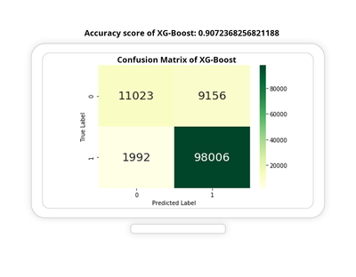
The accuracy score for XG-Boost shows that it’s improved to 90.7%, higher compared to other tree-based techniques.

A confusion matrix has also been drawn for XG-Boost. Here, we can see 98,006 “true positive” values, meaning 98,006 positive reviews are predicted as positive, and only 1,992 positive reviews are predicted as negative reviews (these are called false positives); 98% of positive reviews predicted correctly.

We see 11,023 are “true negatives,” meaning that 11,023 negative reviews were predicted correctly as negative, and 9,156 negative reviews were predicted positive (these are called false negatives); 54.62% of negative reviews were predicted correctly.

We can see both positive and negative review predictions increase with XG-Boost, which leads to the high performance of the model.

4. Clustering

Clustering is an unsupervised ML technique. As the name suggests, it’s a natural grouping or clustering of data. There is no predictive modeling like in supervised learning. Clustering algorithms only interpret the input data and clusters in feature space; there is no predicted label in clustering.

There are some business applications where clustering is widely used:

• Identifying the best-performing members of a company
• Finding the most profitable products
• Finding similar posts or webpages on a website
• Market segmentation 
• Recommendation engines
• Social networking sites
• Customer segmentation based on visitor shopping behavior

K-means clustering 

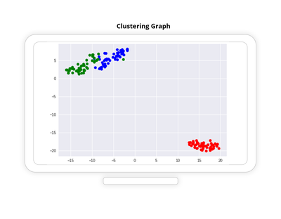
K-means clustering is the most commonly used clustering algorithm. The logic behind k-means clustering works to minimize the variance within each cluster and maximize the variance between the clusters. 

No data point belongs to two clusters. K-means clustering is reasonably efficient in the sense of partitioning of data into different clusters.

Practical applications of clustering:

• Distinguishing customers, e.g., a group of people who tend to buy high-end mobile phones
• Grouping players/students based on their performance

Let’s see the Python code to implement k-means clustering:

from sklearn.cluster import KMeans
BOW_kmeans = KMeans(n_clusters=5, max_iter=100).fit(BOW_train)

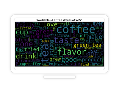
Clustering is very useful in text data, as in text data, each word works as a feature. We can create a word cloud for every cluster to get a sense of how data is partitioned.

Creating a word cloud helps display different clusters with similar kinds of words (words with similar meanings appear near other words) This aids in creating “word embeddings,” a type of word representation that allows words with similar meaning to be understood by machine learning algorithms via mapping them to real number vectors.

Here we have text data of Amazon’s fine food reviews: Let’s see the word clouds for two clusters from our review data (the first cluster is related to beverages, and the second cluster is related to pet food😞

Hierarchical clustering

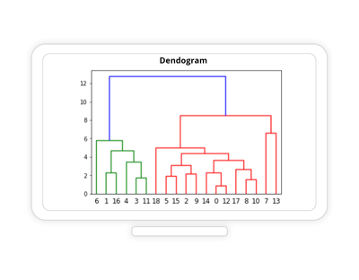
Hierarchical clustering builds a multilevel hierarchy of clusters by creating cluster trees called dendrograms. A horizontal line is used to join the units in the same cluster. It is useful as a visual representation of clusters. Agglomerative clustering is a type of hierarchical clustering.

Practical applications of hierarchical clustering:

• Recognizing a user’s identity via hand biometrics
• Analyzing social media websites to look at which user follows which other users and use that to power a recommendation system

5. Dimensionality reduction

In practical cases, we often have n-dimensional data, which is cumbersome; it’s very time-consuming to deal with high-dimensional data. Dimensionality reduction works to represent data with fewer dimensions by identifying a set of linear combination features that have maximum variance and are mutually uncorrelated. When our dataset has many features, it’s very difficult and time-consuming to analyze.

Most of the information is in the topmost features, so with the help of algorithms, some features that are not useful can be discarded. As in text data, we have many features to deal with, so we can simplify things by dealing with only the features that cover approximately 95% of variance and discard the rest.

With the help of dimensionality reduction techniques, model performance improves.

Practical application of dimensionality reduction:

• Document classification: Classifying documents (with thousands of terms) like reviews, social media posts, emails to different categories
• Facial recognition and medical data classification like MRI classification or tumor detection in images

Both the text and image data are high dimensional, so dimensional reduction improves performance.

Here, we’ll discuss two ideas of dimensionality reduction: principal component analysis (PCA) and latent semantic analysis (LSA).

PCA 

PCA works by transforming the coordinate system of the dataset so that maximal variance is retained. Applying PCA to the vectors of a dataset is like projecting them onto eigenvectors with their corresponding eigenvalues. With PCA, top p eigenvalues are selected and corresponding p eigenvectors taken as new features, and dimensions of data reduced to p. Top p eigenvalues and eigenvectors are selected in such a way that it keeps most of the information intact. It is an unsupervised implementation.

Let’s see Python code implementation of PCA on a Boston house-prices dataset to reduce the dimensions of the dataset from 13 to 2:

from sklearn import decomposition
pca= decomposition.PCA()
# the number of components = 2(Reduce to 2-D data)
pca.n_components = 2
pca_data = pca.fit_transform(train_x)
print("shape of train data = ", train_x.shape)
# pca_reduced will contain the 2-d projects of train data
print("shape of pca_reduced.shape = ", pca_data.shape)

Output: Features dimension reduced from 13 to 2

shape of train data =  (339, 13)
shape of pca_reduced.shape =  (339, 2)

LSA 

Latent semantic analysis is mostly used for textual data. It is a technique to reduce the dimensions of the data that is in the form of a term-document matrix. In a term-document matrix, rows correspond to documents, and columns correspond to terms (words). Term-document matrix is a mathematical matrix that describes the frequency of terms (words) that occur in that row of the document. Here’s a sample term-document matrix: 

	Term
Document	coffee	tasty	very	affordable	love
Coffee is very tasty	1	1	1	0	0
Coffee is very tasty and affordable. Love the coffee	2	1	1	1	1

A term-document matrix of text data is created either by CountVectorizer or TfidfVectorizer, then truncated singular value deposition (SVD). SVD is a method for matrix decomposition from higher dimensions to lower, usually dividing one matrix into three. Applied to a term-document matrix, this transformation is known as LSA. 

Let’s see Python code implementation of LSA on an Amazon fine food reviews dataset to reduce the dimensions of high-featured text data of Amazon fine food reviews:

Truncated svd
from sklearn import decomposition
t_svd= decomposition.TruncatedSVD()
# the number of components = 100(Dimensionaly reduced to 100)
t_svd.n_components = 100
svd_data = t_svd.fit_transform(BOW_train)# BOW_train is term-document-matrix created by CountVectorizer()
print("shape of train data = ", BOW_train.shape)
print("shape of truncated svd = ", svd_data.shape)

Output:

shape of train data =  (243994, 94030)
shape of truncated svd =  (243994, 100)

We can see that the total number of feature dimensions of the matrix has been reduced from 94,030 to 100.

Solving big problems

The solution to every data science problem is unique. Having a working knowledge of a variety of different statistical techniques to use on your non trivial data will allow you to take multiple approaches to get the best results for your challenge. Being armed with the basics of this range of statistical techniques in Python code gives you a great starting point to explore what you can learn from your datasets and how you can train your models to deliver better results.

[EliseWoodard]

This is helpful!