Data Prep Essentials for AI-Driven Analytics - Part 2
Learn how AI training and validation shape reliable models. Explore how structured, diverse data helps AI recognize patterns, generalize effectively, and avoid overfitting—ensuring optimal performance in real-world applications.664Views4likes0Comments
The Sisense Experience: How I Enhanced Data Analytics Leveraging Sisense
Leveraged Sisense to drastically reduce the time from data to insights, enhancing decision-making speed. Utilized Sisense’s robust API for seamless integration and automated most of the actions to standardize implementation Transformed my approach to data analytics, achieving more with less effort through Sisense’s easy-to-use and understand features1.9KViews4likes1CommentPredictive analytics with AutoML for time-series forecasting using Custom Code
Sisense forecasting relies on Sisense’s Cloud Service and machine-learning algorithms. With Sisense, users have the ability to forecast based on historical data in the Sisense widget. Using Custom Code Notebooks, a user can define their input parameters based on their data and train their machine learning model for use as predictive analytics locally meaning without sending the data to Sisense’s Cloud Services.3.3KViews3likes0CommentsData prep essentials for AI-driven analytics - part 3
Discover how to improve data quality for AI and machine learning. In Part 3 of our Data Preparation series, learn how to fix missing values, remove duplicates, correct data types, and standardize formats—with SQL and Python scripts to help you clean your data for accurate, AI-ready analytics.330Views2likes0CommentsAutomated Machine Learning with Sisense Fusion: A Practical Guide
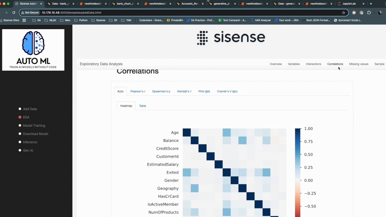
Automated Machine Learning with Sisense Fusion: A Practical Guide In this article, we’ll explore how using Sisense and AutoML (Automated Machine Learning) can simplify the process of applying machine learning to real-world business problems. AutoML takes care of tasks such as data preprocessing, model selection, and hyperparameter optimization without requiring deep expertise in machine learning. Let’s dive into some practical business challenges where machine learning can make a significant impact. Understanding the Business Use Cases To illustrate how machine learning (ML) solves business challenges, we’ll look at two real-world use cases: Optimizing Inventory for a Popular Retail Product (Regression Problem): Imagine a popular clothing store trying to manage stock for a trendy item that frequently sells out. By applying machine learning, the store could predict the future demand for this product. This is an example of a regression problem, where the model forecasts continuous values—such as the number of items to stock—based on historical sales patterns, seasonal trends, and customer behaviors. This allows the store to optimize its inventory, avoid shortages, and maximize sales, demonstrating the power of machine learning to enhance operational efficiencyto stock) based on historical data and other influencing factors. Improving Customer Retention in Subscription Services (Classification Problem): For subscription-based businesses, predicting customer churn is essential. By analyzing data such as usage patterns, customer engagement, and support history, machine learning can predict whether a customer is likely to cancel their subscription. This classification model enables businesses to proactively target at-risk customers with personalized offers or support, helping to improve retention and customer satisfaction. The predictive power of machine learning transforms how businesses engage with their users, reducing churn and increasing long-term loyalty. Difference Between Regression and Classification Regression models are used to predict continuous values, such as quantities (e.g., how many products to stock) or prices. Classification models are used to predict categorical outcomes, such as Yes/No (e.g., whether a customer will churn) or other distinct categories (e.g., fraud/no fraud). Hands-On: Using Sisense Fusion and AutoML Everything demonstrated in this video, including the integration of machine learning models, is powered by Sisense Fusion’s native APIs and features. The web app is simply a wrapper that adds a shiny interface, but all actions performed in the demo—whether selecting data models, training machine learning models, or making predictions—can be done entirely within Sisense Fusion’s native platform without the need for external code or API calls. The power of Sisense Fusion lies in its seamless ability to manage and integrate these machines' learning tasks natively, making it easy for users to build, deploy, and interact with models without needing deep technical expertise or external integrations. The web app just provides a visually engaging way to demonstrate the capabilities of the Sisense Fusion platform. Step 1: Selecting the Data Model and Dataset In the first part of the video, we use the web app that leverages Sisense Fusion’s native API features to select the data model we want to work with. Here’s a breakdown of what happens: Selecting a Data Model: After starting the app, we selected the data model available in Sisense that contains our data. Choosing the Dataset: Once the data model is selected, the app displays all the tables or datasets contained in that model. We then select the dataset we want to train the machine learning model on. Target Variable Selection: After selecting the dataset, the app presents all the columns within the dataset. We select the target variable (the column we want to predict). For example, in customer churn prediction, this could be the Exited column, which indicates whether a customer has churned (1) or not (0). Selecting the Prediction Type: Next, we select whether the task is a regression or classification problem, based on the target variable. Since we are predicting customer churn, we select a classification. Storing Information: Once all selections are made, the app stores this information. This data will later be used when we select the machine learning model for training. Step 2: Exploratory Data Analysis (EDA) After submitting behind the scenes, a Flask application generates an Exploratory Data Analysis (EDA) report based on the dataset. This report provides important insights, such as: Number of customer records. Missing values in the dataset. Relationships between variables. These insights help us select relevant columns to ensure the machine learning model performs optimally. Step 3: Model Training Options We can have multiple options for training our model within Sisense Fusion for example: Auto-Sklearn: This is an open-source AutoML library that automates the model training process. Since it runs locally within Sisense, data never leaves the platform, ensuring data security. However, model training can be computationally expensive, meaning your Sisense cluster should have adequate resources to handle it. AWS Autopilot: This option leverages Amazon Web Services (AWS) infrastructure to train the model, offering more reliable performance. However, it incurs additional costs and requires your data to be sent to AWS for processing. After selecting the model training method, the process begins automatically, and you’ll see the status on the screen as it progresses. Part 4: Integration with AWS SageMaker and Dashboard Creation After selecting the AWS option for model training in the web app a new Custom Code Table is added to the Sisense data model. This Custom Code Table automates the training and deployment of the machine learning model using AWS SageMaker Autopilot. Here’s how it works: Input Parameters for the Notebook The custom code notebook contains a set of input parameters that are passed based on the selections made earlier in Part 1 (dataset and target column). Other parameters include: Dataset: The table you selected for model training. Target Column: The data column you want to predict (churn, in this case). Drop Feature: Columns you wish to exclude from model training (optional). AWS Credentials: Paths to AWS access keys and secret keys to authenticate with AWS. S3 Bucket Name: A unique S3 bucket where the dataset is stored for training. AWS Role ARN: The role with the necessary permissions to access S3 and SageMaker. The notebook code reads these parameters and uses them to call the AWS SageMaker Autopilot API, which automates the model training and deployment process. The trained model is deployed as an endpoint on SageMaker, allowing for online predictions. Creating a Blox widget with dynamic input fields The custom code notebook also contains code that dynamically creates a Sisense dashboard and a Blox widget based on the dataset selected for model training. Here’s what happens: Dynamic Input Fields: Based on the feature columns in the dataset, the Blox widget dynamically generates input fields (boxes) for each feature. This is crucial for online predictions, as it allows users to input new data for the model to predict outcomes in real time. Predict Button: A predict button is added to the widget. When a user inputs new data into the input boxes and clicks the predict button, the system requests the SageMaker endpoint, passing the input data. The model processes this data and returns the prediction, which is displayed in the widget. This setup enables real-time, online predictions directly from the Sisense dashboard, with predictions being powered by the AWS SageMaker endpoint. The dynamic nature of the widget allows the interface to adjust based on the dataset used for training, making the system flexible and user-friendly. The custom code table outputs key information about the trained model and its deployment status, which includes the following columns: Model Name: The name assigned to the trained machine learning model. Metric Name: The evaluation metric used to assess the model's performance, such as accuracy, precision, or recall. Score: The metric score that indicates how well the model performed during evaluation. Local Path: The path within the Sisense environment where the model is stored. Model S3 Location: The S3 location where the trained model is saved after deployment. AWS Model Name: The name of the model is registered in AWS SageMaker. Endpoint Name: The name of the deployed SageMaker endpoint used for making real-time predictions. This output allows users to track key details about the model, including where it's stored, its performance, and the endpoint used for predictions. Step 5: Saving Model Versions The notebook not only trains the model but also saves important metadata within Sisense’s file management storage. This allows you to maintain version control over your models. For each model training session, I store details such as the model metrics (accuracy, precision, etc.) and save each model in a folder based on the timestamp. This ensures easy traceability and allows for multiple versions of models to be stored and retrieved as needed. Step 6: Making Predictions Once the model is trained, we move on to predictions. There are two ways to handle predictions: Batch Predictions (Offline): This method allows you to process thousands of records at once. It's suitable for scenarios where real-time predictions are not required, and predictions can be generated in bulk. Online Predictions (Real-Time): For real-time applications, you can provide individual customer records and receive immediate predictions. This is ideal for real-time decision-making, such as predicting whether a new customer will churn based on their current attributes. Online Predictions (Real-Time): When a custom code table was built it automatically generated a Sisense dashboard and a Blox widget based on the input features used during model training. This integration allows predictions to be embedded directly into Sisense dashboards, enabling users to interact with the model seamlessly. Here’s how it works: The Blox widget takes the input data from the user and sends an API request to Sisense’s custom code transformation. In the case of Auto-Sklearn, the pre-trained model is loaded locally within Sisense, as the model was trained and stored in the local environment. For AWS SageMaker, instead of loading a local model, the system sends a request to the SageMaker endpoint (where the model is deployed) for predictions. The prediction results, whether generated locally with Auto-Sklearn or through the SageMaker API, are returned to the dashboard and displayed within the Blox widget in real-time. This process ensures that predictions are fully integrated into the Sisense environment, providing an interactive and real-time experience for users, with the flexibility to use either local or cloud-based models depending on their needs. Conclusion Sisense Fusion, combined with AutoML, offers an efficient and powerful way to integrate machine learning into real-world business applications. Whether using Auto-Sklearn for local, cost-efficient model training or AWS Autopilot for cloud-based scalability, Sisense provides seamless version control and easy integration into dashboards, making it a comprehensive platform for automating machine learning at scale. If you’re interested in integrating this solution into your Sisense deployment, please reach out to your dedicated Customer Success Manager (CSM) for further assistance. Related Content: https://docs.sisense.com/main/SisenseLinux/ai-overview.htm https://academy.sisense.com/gen-ai Related Content:2.9KViews2likes0Comments
Introduction To Hyperparameter Optimization - Machine Learning
There are lots of knobs (a.k.a hyperparameters) we can turn when coming up with a Machine Learning model. in the script below, we take the well-known iris dataset, and play around with different hyperparameters. First, a few notes: In machine learning, we generally split our data into 3 sections A training dataset A dev dataset A test dataset We train the model on the training dataset, tune hyperparameters based on the dev dataset, and only run the test dataset when we're evaluating our model. Note that we don't want to tune hyperparameters based on the output of our test dataset in order to avoid overfitting both the test and training dataset if you want to quickly iterate through many different hyperparameters, I recommend using a smaller subset of your data to allow for quick processing. Once some of the hyperparameters have been narrowed down, you can dedicate more time and computational resources to running the full training dataset and creating the model in your production workflow. Without further ado, here is a hyperparameter optimization on K Nearest Neighbors using the corresponding classifier from the Python sklearn library. The below example uses Python 3.6 code. First, we import our libraries: import pandas as pd import numpy as np from sklearn.model_selection import train_test_split from sklearn.datasets import load_iris from sklearn.neighbors import KNeighborsClassifier from sklearn.utils import shuffle from sklearn.metrics import f1_score import matplotlib.pyplot as plt import random I set a random.seed() here to make results reproducible random.seed(123) In this example, we are building a dataframe which contains the iris dataset. However, for your own purposes, you can very well use your SQL output, which will get passed into the Sisense for Cloud Data Teams Python/R editor as a dataframe named df. Your final dataframe must have a list of features (these are the predictor components, you can think of these as your "X," and the corresponding label, you can think of this as your "y"). This dataframe below has 3 features: the sepal length, sepal width, and petal length. We also have a column, 'target,' which contains the name of the iris type. iris = load_iris() df = pd.DataFrame(data= np.c_[iris['data'], iris['target']], columns= iris['feature_names'] + ['target']) df = df.drop('petal width (cm)', axis = 1) Next, we shuffle the dataframe to ensure we are getting a representative sample of our data in the training, dev, and test dataset. df = shuffle(df, random_state = 300) Now, we want to split our target column (y) from all of our features (our x values) df_features = df.drop('target', axis = 1) features = df_features.values target = df["target"].values Now we split our data into training, dev, and test datasets num_rows = df.shape[0] train_cutoff = int(num_rows * 0.6) dev_cutoff = int(num_rows * 0.8) features_train = features[:train_cutoff,:] features_dev = features[train_cutoff:dev_cutoff,:] features_test = features[dev_cutoff:,:] target_train = target[:train_cutoff] target_dev = target[train_cutoff:dev_cutoff] target_test = target[dev_cutoff:] Now, we loop through all our hyperparameters. In this example, we are looping through all values of n_neighbors from 1 to 10. This determines how many of our "neighbors" we are using to classify a given point outside our training dataset. Additionally, we will compare the effectiveness of using "uniform" versus "distance" weights for our model. Note that: A "uniform" weight takes a vote between the N closest neighbors of a point to classify it. A "distance" weight gives more importance to those neighbors that are closest to the point. For example, let's say our KNN is looking at n_neighbors of 5. if of the 5 closest neighbors, the closest of them all is Category A, that will be given more weight than the furthest of the 5 neighbors. To evaluate the dataset, we will run a .predict() function on model using the dev dataset, and score the model using the F1 score (F1 is better at capturing false positives and false negatives, more info on this here). Note that you can achieve this logic with GridSearchCV as well all_k = range(1,11) uniform = [] distance = [] # Looping through all values of k for nbrs in all_k: knn_uni = KNeighborsClassifier(n_neighbors = nbrs, weights = 'uniform') knn_dist = KNeighborsClassifier(n_neighbors = nbrs, weights = 'distance') pred_uni = knn_uni.fit(features_train, target_train).predict(features_dev) pred_dist = knn_dist.fit(features_train, target_train).predict(features_dev) f1_uni = f1_score(target_dev, pred_uni, average = 'macro') f1_dist = f1_score(target_dev, pred_dist, average = 'macro') uniform.append(f1_uni) distance.append(f1_dist) Finally, we plot our results fig, (ax1, ax2) = plt.subplots(1, 2, sharey=True) ax1.plot(all_k, uniform) ax1.set_title('Uniform Weights') ax1.set_ylabel('F1 Score') ax2.plot(all_k, distance) ax2.set_title('Distance Weights') # Use Sisense for Cloud Data Teams to visualize a dataframe, text, or an image by passing data to periscope.table(), periscope.text(), or periscope.image() respectively. periscope.image(fig) Now we analyze the output. The number of neighbors used to generate the model is on the x axis, with the F1 score on the y axis. An F1 score closer to 1 is more desirable here. We see that there are more fluctuations in the uniform weights scoring compared to the distance weights. This is expected as we would anticipate the closest neighbors to be more informative when classifying an iris. Therefore, distance weights looks like a better option. Secondly, it looks like distance weights with 6-8 neighbors yield the highest F1 score. We would go on the lower end of our range here as n_neighbors of 6 is less computationally intensive than n_neighbors of 8 (we have fewer neighbors to account for when classifying each point). Of course, we used a very very small dataset here, so we can expect the lines above to be smoother for a larger dataset. Any other parameters you like to play around with for KNN? Now that we have found our desired hyperparameters, let's run this on our test dataset! Let's put this in a Sisense for Cloud Data Teams view so it's easy to leverage this logic multiple times without rewriting code. See post here for further details!1.2KViews1like0Comments